Low-rank approximation 2/4
Tech
Overview of Low-rank approximation – Part2
1. Matrix Decomposition Techniques
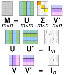
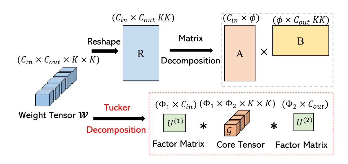
Singular Value Decomposition (SVD): SVD is a linear algebra technique that decomposes a matrix into three other matrices. For a convolutional filter represented as a matrix \(W\), SVD finds matrices \(U\), \(\Sigma\), and \(V\) such that \(W = U \Sigma V^T\).
- Application: By keeping only the top \(k\) singular values from \(\Sigma\), and the corresponding columns in \(U\) and \(V\), we can create a low-rank approximation of the original filter.
- Benefits: This significantly reduces the number of parameters and computations involved.
Tucker Decomposition: Tucker decomposition generalizes SVD for tensors (multi-dimensional arrays). It decomposes a tensor into a core tensor and a matrix factorization of each mode (dimension).
- Application: In CNNs, filters can be represented as 3D tensors (width, height, depth). Tucker decomposition approximates the filter as a smaller core tensor with smaller matrices for each dimension.
- Benefits: Allows a more flexible approximation with potentially better representation capabilities compared to SVD.
- CP (CANDECOMP/PARAFAC) Decomposition: CP decomposition also approximates a tensor by expressing it as the sum of a finite number of rank-one tensors.
- Application: In CNNs, it can help decompose filters into simpler components that capture the same information with fewer parameters.
- Benefits: It can be simpler to implement in certain situations than Tucker decomposition.
2. Filter Factorization Techniques
- Two-Dimensional Factorization: Instead of using one large convolutional kernel, it decomposes it into two smaller kernels, typically one for spatial dimensions (width and height) and one for the depth dimension.
- Application: A \(k \times k \times d\) filter can be approximated by multiplying a \(k \times k\) filter with a \(k \times 1\) filter for each depth slice.
- Benefits: This reduces the computational complexity from \(O(k^2 \cdot d)\) to \(O(k^2 + k \cdot d)\).
- Depthwise Separable Convolutions: This technique separates the convolution process into two layers: a depthwise convolution (applies a single filter per input channel) followed by a pointwise convolution (1x1 convolution to combine the outputs).
- Application: MobileNets, for instance, use this technique extensively to reduce the number of parameters while maintaining performance.
- Benefits: It reduces both computational and memory requirements significantly compared to standard convolutions.
3. Quantization Techniques
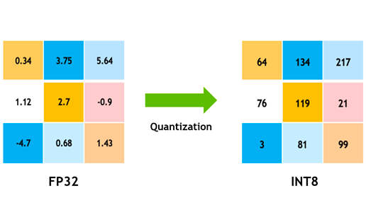
Weight Quantization: Involves reducing the precision of the weights (e.g., using 8-bit integers instead of 32-bit floating-point numbers).
- Application: After performing low-rank approximation, quantization can further reduce the model size and speed up inference on hardware with limited precision.
- Benefits: Lower memory usage and faster computation, especially on specialized hardware like GPUs or TPUs.
4. Structured Low-Rank Approximations
- Low-Rank Convolutional Filters: Instead of fully dense filters, structured filters with fewer connections can be designed to maintain performance while reducing rank.
- Application: This may involve using predefined patterns or structures for the filters based on the spatial hierarchies present in the data.
- Benefits: More efficient use of parameters while exploiting spatial correlation in images.
5. Regularization Techniques
- Low-Rank Regularization: Adding a low-rank regularization term to the loss function during training encourages the network to learn low-rank filters.
- Application: This could be achieved by penalizing the nuclear norm (sum of singular values) of the filter matrices in the loss function.
- Benefits: Helps in obtaining low-rank approximations directly from the training process, maintaining a good trade-off between accuracy and model size.


